1. AnnoyClassifier¶

1.1. Importing Packages¶

from mlots.models import AnnoyClassifier
from sklearn.model_selection import GridSearchCV
from scipy.io import arff
import matplotlib.pyplot as plt
import pandas as pd
import numpy as np
import warnings
from sklearn.metrics import accuracy_score
warnings.filterwarnings("ignore")
import matplotlib
%matplotlib inline

font = {'size'   : 22}

matplotlib.rc('font', **font)

1.2. Loading Data¶

Here we are loading the SmoothSubspace dataset.
The datasets are in two .arff files with pre-defined train and
test splits.
The following code reads the two files stores the X (time-series
data) and y (labels), into their specific train and test sets.
***

name = "SmoothSubspace"

dataset = arff.loadarff(f'../input/{name}/{name}_TRAIN.arff'.format(name=name))[0]
X_train = np.array(dataset.tolist(), dtype=np.float32)
y_train = X_train[: , -1]
X_train = X_train[:, :-1]

dataset = arff.loadarff(f'../input/{name}/{name}_TEST.arff'.format(name=name))[0]
X_test = np.array(dataset.tolist(), dtype=np.float32)
y_test = X_test[: , -1]
X_test = X_test[:, :-1]

#Converting target from bytes to integer
y_train = [int.from_bytes(el, "little") for el in y_train]
y_test = [int.from_bytes(el, "little") for el in y_test]
X_train.shape, X_test.shape

((150, 15), (150, 15))

Set	Sample size	TS length
Train	150	15
Test	150	15

1.3. Evaluating AnnoyClassifier¶

1.3.1. Default parameters¶

We would employ AnnoyClassifier model from the mlots python package.

First, the model is evaluated with default parameters over the SmoothSubspace dataset. ***

model_default = AnnoyClassifier(random_seed=42).fit(X_train,y_train)

y_hat_default = model_default.predict(X_test)
acc_default = accuracy_score(y_test, y_hat_default)
print("Model accuracy with default parameters: ", round(acc_default, 2)*100)

Model accuracy with default parameters:  87.0

The accuracy of the model is 87%, which is already a good classification accuracy. However, lets see if we can squeeze in more effective performance.

1.3.2. Model tuning¶

AnnoyClassifier model allows us to work with a more complex
distance measure like DTW in a MAC/FAC strategy.
Here, we would use GridSearchCV algorithm from the sklearn
package to find the best set of parameters of the model over the
dataset.
The model tuning would be done only over the train set of the
dataset. ***

#Setting up the warping window grid of the DTW measure

dtw_params = []
for w_win in range(1,6,2):
    dtw_params.append(
    {
        "global_constraint": "sakoe_chiba",
        "sakoe_chiba_radius": w_win
    }
    )
dtw_params

[{'global_constraint': 'sakoe_chiba', 'sakoe_chiba_radius': 1},
 {'global_constraint': 'sakoe_chiba', 'sakoe_chiba_radius': 3},
 {'global_constraint': 'sakoe_chiba', 'sakoe_chiba_radius': 5}]

#Setting up the param grid for the AnnoyClassifier model with the DTW params

param_grid = {
    "n_neighbors": np.arange(1,12,2),
    "mac_neighbors": np.arange(15,50,5),
    "metric_params" : dtw_params
}
param_grid

{'n_neighbors': array([ 1,  3,  5,  7,  9, 11]),
 'mac_neighbors': array([15, 20, 25, 30, 35, 40, 45]),
 'metric_params': [{'global_constraint': 'sakoe_chiba',
   'sakoe_chiba_radius': 1},
  {'global_constraint': 'sakoe_chiba', 'sakoe_chiba_radius': 3},
  {'global_constraint': 'sakoe_chiba', 'sakoe_chiba_radius': 5}]}

#Executing the GridSearchCv over the AnnoyClassifier model with the supplied param_grid.

model = AnnoyClassifier(random_seed=42)
gscv = GridSearchCV(model, param_grid=param_grid, cv=5,
                    scoring="accuracy", n_jobs=-1).fit(X_train,y_train)

#Displaying the best parameters of AnnoyClassifier within the search grid.

best_param = gscv.best_params_
best_score = gscv.best_score_
print("Best Parameters: ", best_param)
print("Best Accuracy: ", best_score)

Best Parameters:  {'mac_neighbors': 45, 'metric_params': {'global_constraint': 'sakoe_chiba', 'sakoe_chiba_radius': 1}, 'n_neighbors': 11}
Best Accuracy:  0.9933333333333334

1.3.3. Evaluation of tuned model¶

The parameters displayed above are optimal set of parameters for the AnnoyClassifier model over SmoothSubspace dataset.

Our next task is then to train the AnnoyClassifier model over the train set with the optimal set of parameters, and evaluate the model over the held-out test set. ***

model_tuned = AnnoyClassifier(**best_param,random_seed=42).fit(X_train,y_train)

y_hat_tuned = model_tuned.predict(X_test)
acc_tuned = accuracy_score(y_test, y_hat_tuned)
print("Model accuracy with tuned parameters: ", round(acc_tuned, 2))

Model accuracy with tuned parameters:  0.98

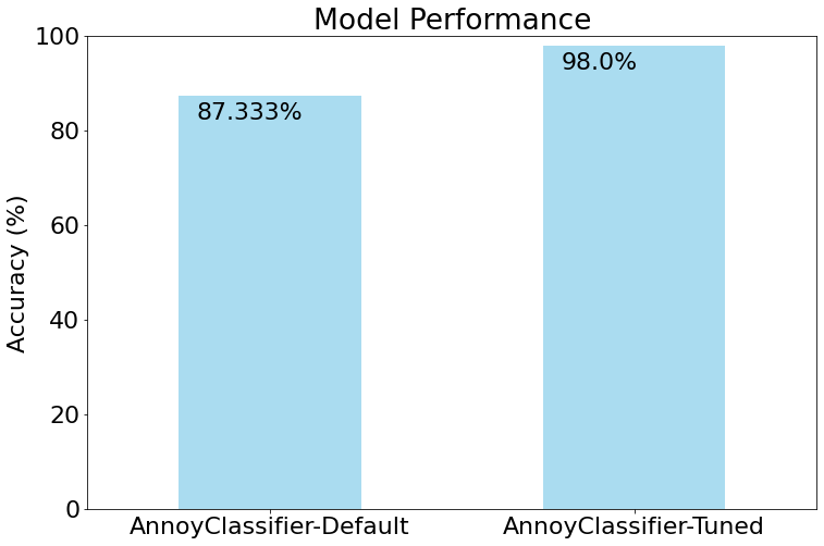
By tuning the parameters of the model we increased the accuracy of the model from ~\(87\)-\(90\%\) to \(98\%\).

1.4. Comparison¶

Here we do bar-plot that would illustrate the performance of the AnnoyClassifier model with default parameters against the model with the tuned parameters.

The matplotlib.pyplot is employed for this task. ***

acc =  [acc_default*100,acc_tuned*100]
rows = ["AnnoyClassifier-Default", "AnnoyClassifier-Tuned"]

df = pd.DataFrame({"models": rows, "Accuracy":acc})

fig = plt.figure()
ax = df['Accuracy'].plot(kind="bar", figsize=(12, 8), alpha=0.7,
                 color=[
                     'skyblue'
                 ], label = "Accuracy")

ax.set_xticklabels(df['models'])
ax.set_ylabel("Accuracy (%)")

ax.set_ylim(0,100)

plt.setp(ax.xaxis.get_majorticklabels(), rotation=0)
for i,a in enumerate(acc):
    ax.text(i-0.2,a-5,str(round(a,3))+"%")
plt.text
plt.title("Model Performance")
plt.show()